
Learning Center
How to fit an Arima model to a time series?
The ARIMA model was invented in 1976 by the statisticians Box and Jenkins, being considered one of the most useful methods to forecast a time series.
Fitting an ARIMA(p,d,q) model into a time series is a matter of choosing the order p for the autoregressive parameters, the order q for the moving average parameter and the number d of differences to be applied in the time series. In practice, this is made by looking the correlogram of the time series and inferring the parameters p, d and q that makes the correlogram of residuals not significant at any lags. To clarify this process an example will be given.
Example
Considering the time series below, fit an ARIMA model into it.
A |
B |
C |
D |
E |
F |
|
1 |
3-month Treasury bill (secondary market rate) |
|
|
|
|
|
2 |
|
|
|
|
|
|
3 |
1990-01 |
7.64 |
|
|
|
|
4 |
1990-02 |
7.74 |
|
|
|
|
5 |
1990-03 |
7.9 |
|
|
|
|
6 |
1990-04 |
7.77 |
|
|
|
|
7 |
1990-05 |
7.74 |
|
|
|
|
8 |
1990-06 |
7.73 |
|
|
|
|
9 |
1990-07 |
7.62 |
|
|
|
|
10 |
1990-08 |
7.45 |
|
|
|
|
11 |
1990-09 |
7.36 |
|
|
|
|
12 |
1990-10 |
7.17 |
|
|
|
|
13 |
1990-11 |
7.06 |
|
|
|
|
14 |
1990-12 |
6.74 |
|
|
|
|
... |
... |
... |
|
|
|
|
301 |
2014-11 |
0.02 |
|
|
|
|
302 |
2014-12 |
0.03 |
|
|
|
|
303 |
2015-01 |
0.03 |
|
|
|
|
304 |
2015-02 |
0.02 |
|
|
|
|
305 |
2015-03 |
0.03 |
|
|
|
|
306 |
2015-04 |
0.02 |
|
|
|
|
307 |
2015-05 |
0.02 |
|
|
|
|
308 |
2015-06 |
0.02 |
|
|
|
|
309 |
2015-07 |
0.03 |
|
|
|
|
310 |
2015-08 |
0.07 |
|
|
|
|
311 |
2015-09 |
0.02 |
|
|
|
|
312 |
2015-10 |
0.02 |
|
|
|
|
313 |
2015-11 |
0.12 |
|
|
|
|
314 |
2015-12 |
0.23 |
|
|
|
|
315 |
|
|
|
|
|
|
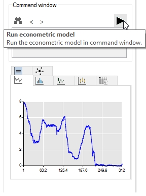
The first step before entering in any statistical procedure is to plot the time series and visualize any significant pattern. To do it using SAFE TOOLBOXES®, just go to the econometrics task pane, select any point of the time series and press the green arrow button. Automatically this line chart will appear at the bottom of the pane:
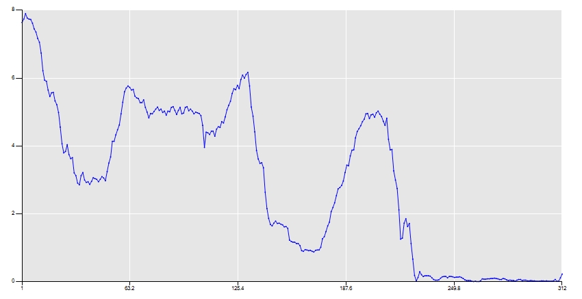
To better visualize the series you can just double click the chart in order to expand it.
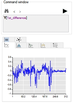
The ARIMA model is useful to a stationary series, that is, a series with a mean and variance that do not change over time. In the above series, is worth trying to remove the trend of the time series applying some degree of differentiation. Entering the command Y[1st_difference] in the command box and clicking on the green arrow button, the chart of the series after applying the first difference will appear:
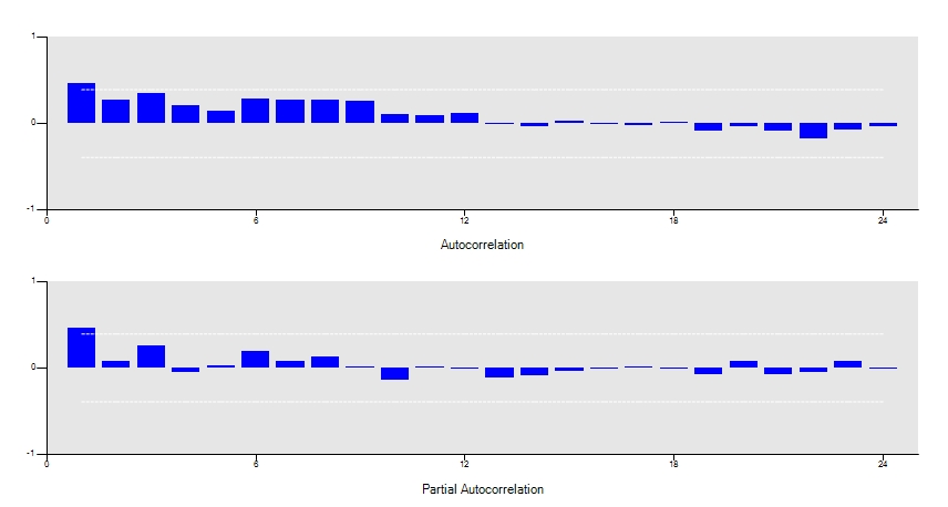
Now, it looks like the trend has been removed and the ARMA terms can be safely applied. To guess an appropriate order of the terms, select the correlogram tab ![]() and check for isolated significant lags in the ACF and the PACF graphs. As a rule of thumb, the number of the isolated lags in the PACF will give the order of AR terms and/or the number of the isolated lags in the ACF will give the order of the MA terms.
and check for isolated significant lags in the ACF and the PACF graphs. As a rule of thumb, the number of the isolated lags in the PACF will give the order of AR terms and/or the number of the isolated lags in the ACF will give the order of the MA terms.
Now, with your initial guess for the p, d and q terms, you can enter the command ARIMA(p,d,q) replacing the p, d and q terms, for instance, 'ARIMA(1,1,1)' and an ARIMA(1,1,1) model will be fitted. Then, it’s important to check the plot of actual vs. predicted, the plot of the residuals (right clicking the actual vs predicted plot and choosing the residuals option), the correlogram of the residuals (again, right clicking the correlogram plot and choosing the residuals option) and the model table (available in the tab ![]() ).
).
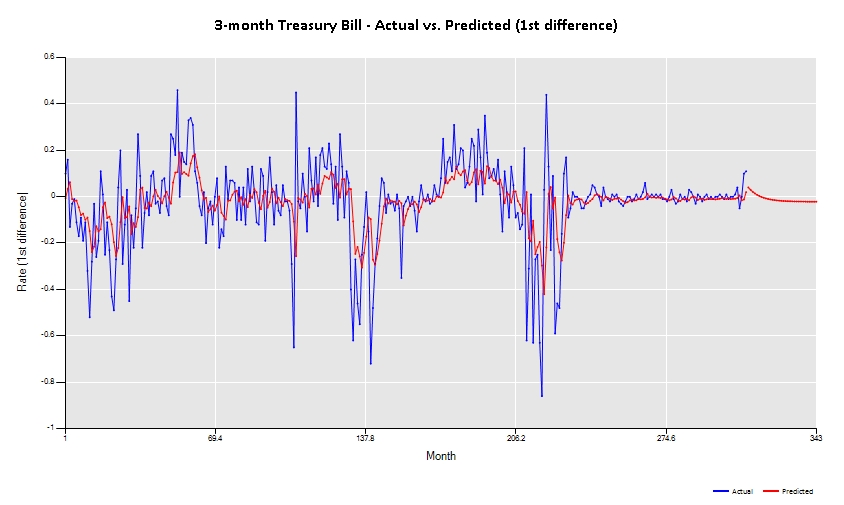
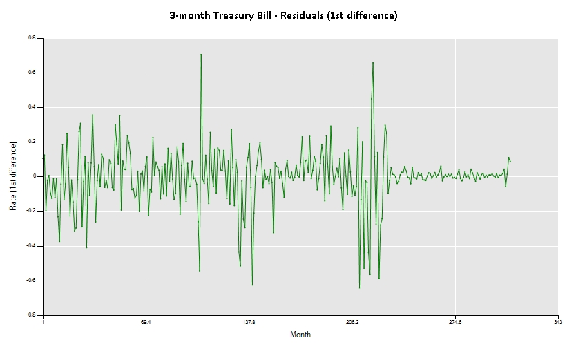
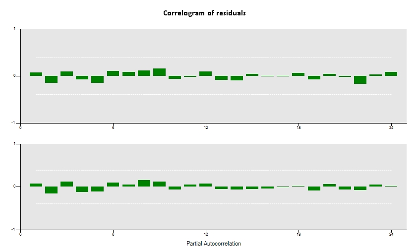
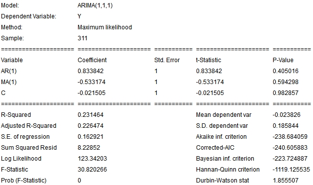
A successful model will present a very close actual vs. predicted plot, a correlogram of residuals without significant lags and statistically significant explanatory variables.
Later on, you can also test the model with different p, d and q parameters and to help you decide which model better suit your data, you can check in the tab ![]() the one that has the minimum value of the Akaike inf. criterion(AIC), Corrected AIC, Bayesian inf. criterion (BIC) or Hannan-Quinn criterion. Also, if you are reserving some part of the data to be used for out of sample tests, you can choose the one that presents the minimum value of the forecast Mean Absolute Deviation (MAD), forecast Mean Absolute Deviation (MAD) or forecast Root of Mean Square Error (RMSE).
the one that has the minimum value of the Akaike inf. criterion(AIC), Corrected AIC, Bayesian inf. criterion (BIC) or Hannan-Quinn criterion. Also, if you are reserving some part of the data to be used for out of sample tests, you can choose the one that presents the minimum value of the forecast Mean Absolute Deviation (MAD), forecast Mean Absolute Deviation (MAD) or forecast Root of Mean Square Error (RMSE).
Finally, you should note that as the majority of SAFE TOOLBOXES® procedures, the ARIMA model can be inserted directly in Excel through the usage of the spreadsheet functions “sTimeSeriesARIMA_Model” that returns the model estimation table and the function “sTimeSeriesARIMA_Predicted” that returns the predicted values by the model.
