Learning Center
How to fit a general equilibrium to model asset returns?
The Financial Toolbox implements two great theoretical models that give the general equilibrium expected return for every asset in the economy. In this toolbox, you can found the Capital Asset Pricing Model (CAPM), developed by Treynor, Sharpe, Lintner and Mossin in the sixties and the Arbitrage Pricing Theory (APT) model, proposed by Ross in 1976.
First of all, it’s worth mentioning that despite the theoretical models mentioned the word “price” in their names, the theory is very applicable to “returns”, since expected future prices are tightly related to the concept of expected returns. The following equations show how you can get the expected returns for a given asset i under the two methodologies:
- Expected return CAPM: ri = rf + β(rm-rf)
- Expected return APT (version 1): ri =ai + b1F1 + b2F2 + … + bnFn
Where, ri is the expected return of the asset i, rf is the risk-free asset, rm is the return of the market portfolio, ai is a constant, β is the sensitivity of the asset to the market excess returns, bj is the sensitivity of the asset to factor Fj. In the APT model, each factor Fj is a weighted basket of explanatory variables for asset returns. Those factors are uncorrelated since they are calculated through the principal components analysis technique. As the factors Fj does not have an explicit economic significance, it’s better to map them back to the explanatory variables. This leads to the following equation for the expected return:
- Expected return APT (version 2): ri =rf + β1(r1-rf) + β2(r2-rf) + … + βm(rp-rf)
Where βi is the sensibility for the explanatory variable rj-rf.
Therefore, given rf and the historical series for ri and rm (for the CAPM) or r1, … , rp (for the APT) fitting an equilibrium model is a matter of estimating the parameters β (for CAPM) or β1, …, βm (for APT). The following examples illustrate how easy it is to use the Financial Toolbox to fit the parameters for a list of assets.
Let’s first start with a sample time series of two stocks and the time series of the explanatory variables used to explain the returns of the stocks.
A |
B |
C |
D |
E |
F |
|
1 |
|
Apple Inc. |
Exxon Mobil Corporation |
S&P 500 |
Consumer Price Index (USA) |
Crude Oil Price (WTI) |
2 |
Jan-11 |
0.052 |
0.103 |
0.023 |
0.005 |
0.000 |
3 |
Feb-11 |
0.041 |
0.066 |
0.032 |
0.005 |
-0.007 |
4 |
Mar-11 |
-0.013 |
-0.016 |
-0.001 |
0.010 |
0.161 |
5 |
Apr-11 |
0.005 |
0.046 |
0.028 |
0.006 |
0.065 |
6 |
May-11 |
-0.007 |
-0.046 |
-0.014 |
0.005 |
-0.079 |
7 |
Jun-11 |
-0.035 |
-0.025 |
-0.018 |
-0.001 |
-0.046 |
8 |
Jul-11 |
0.163 |
-0.020 |
-0.021 |
0.001 |
0.011 |
9 |
Aug-11 |
-0.014 |
-0.066 |
-0.057 |
0.003 |
-0.113 |
10 |
Sep-11 |
-0.009 |
-0.019 |
-0.072 |
0.002 |
-0.009 |
11 |
Oct-11 |
0.062 |
0.075 |
0.108 |
-0.002 |
0.009 |
12 |
Nov-11 |
-0.056 |
0.036 |
-0.005 |
-0.001 |
0.126 |
13 |
Dec-11 |
0.060 |
0.054 |
0.009 |
-0.002 |
0.014 |
14 |
Jan-12 |
0.127 |
-0.012 |
0.044 |
0.004 |
0.017 |
... |
... |
... |
... |
... |
... |
... |
48 |
Nov-14 |
0.106 |
-0.057 |
0.025 |
-0.005 |
-0.102 |
49 |
Dec-14 |
-0.072 |
0.021 |
-0.004 |
-0.006 |
-0.218 |
50 |
Jan-15 |
0.061 |
-0.054 |
-0.031 |
-0.005 |
-0.204 |
51 |
Feb-15 |
0.101 |
0.020 |
0.055 |
0.004 |
0.071 |
52 |
Mar-15 |
-0.031 |
-0.040 |
-0.017 |
0.006 |
-0.055 |
53 |
Apr-15 |
0.006 |
0.028 |
0.009 |
0.002 |
0.139 |
54 |
May-15 |
0.045 |
-0.017 |
0.010 |
0.005 |
0.089 |
55 |
Jun-15 |
-0.037 |
-0.023 |
-0.021 |
0.004 |
0.009 |
56 |
Jul-15 |
-0.033 |
-0.048 |
0.020 |
0.000 |
-0.149 |
57 |
Aug-15 |
-0.066 |
-0.041 |
-0.063 |
-0.001 |
-0.158 |
58 |
Sep-15 |
-0.022 |
-0.012 |
-0.026 |
-0.002 |
0.061 |
59 |
Oct-15 |
0.083 |
0.113 |
0.083 |
0.000 |
0.016 |
60 |
Nov-15 |
-0.006 |
-0.004 |
0.001 |
-0.002 |
-0.082 |
61 |
Dec-15 |
-0.110 |
-0.045 |
-0.018 |
-0.003 |
-0.124 |
62 |
|
|
|
|
|
|
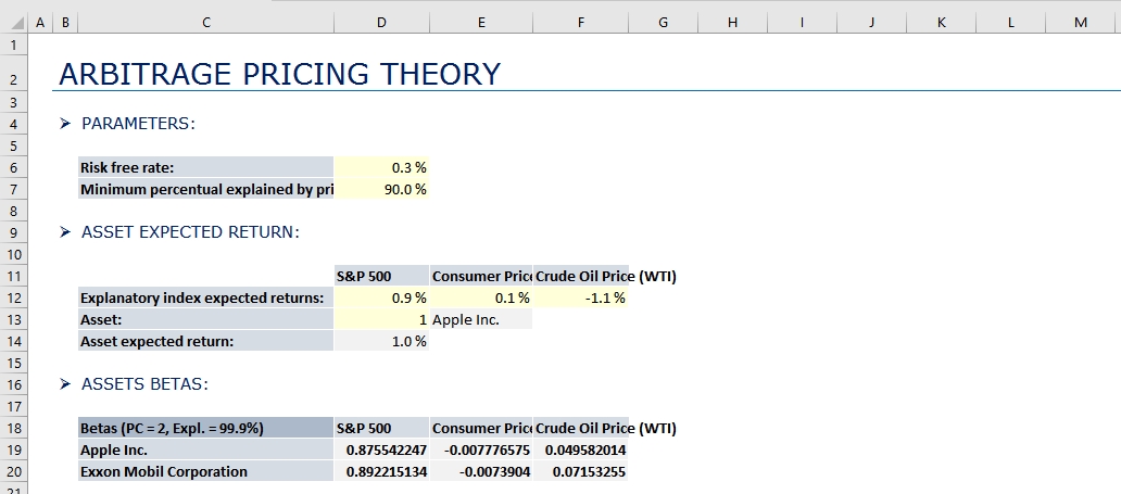
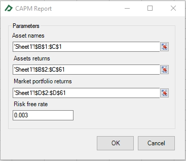
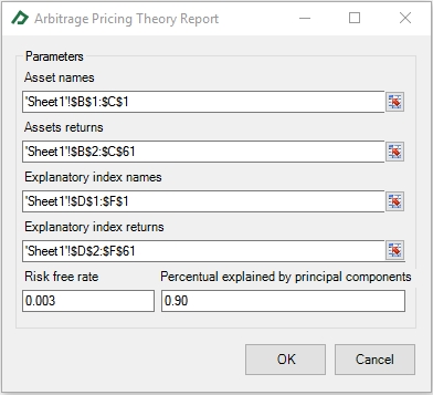
Supposing that the risk-free rate is 0.3% per month, that the S&P 500 is the right proxy for the market portfolio in the CAPM model and the series of S&P 500, Consumer Price Index (USA), and the Crude Oil Price (WTI) are the explanatory variables in the APT model. You can select the corresponding option in the “Market” group of the Financial Toolbox tab and set up them as following:
The result of the procedures is displayed in new sheets (see below). The fitted coefficients can be used to infer the expect returns of the stocks using the functions “sCAPM_ExpectedReturn” and “sAPT_ExpectedReturn”.