Learning Center
How to calculate the liability and cash flows for a retirement benefit?
In this example we are going to show how to calculate the liability and the predicted cash flows for a retirement benefit for an individual in a pension fund. A determinist and a stochastic version of the calculus for a pension scheme that includes a regular retirement income, a disability income, a death pension benefit and a life insurance will be presented below.
|
A |
B |
C |
1 |
Pension liability example: |
|
|
2 |
|
|
|
3 |
Retired contribution |
0.05 |
|
4 |
Worker contribution rate over gross salary |
0 |
|
5 |
Worker contribution rate over net salary (gross - social security) |
0.1 |
|
6 |
Administrative costs |
0.1 |
|
7 |
Current gross salary (annual) |
100000 |
|
8 |
Current age |
30 |
|
9 |
Retirement age |
65 |
|
10 |
Growth (real) rate of worker salary |
0.03 |
|
11 |
Growth (real) rate of retired pension |
0 |
|
12 |
Disability entrance table |
80 |
|
13 |
Life table normal life |
6 |
|
14 |
Life table disabled life |
2 |
|
15 |
Current Social Security reference benefit (annual) |
30000 |
|
16 |
Growth (real) rate of Social Security reference benefit |
0.01 |
|
17 |
Is normal |
TRUE |
|
18 |
Forward (real) interest rate curve |
0.05 |
|
19 |
Life table dependent |
1 |
|
20 |
Expected inflation rate |
0.05 |
|
21 |
Life insurance benefit (% over salary) |
0.083333333 |
|
22 |
Age at wedding |
27 |
|
23 |
Children maximum age to receive benefits |
20 |
|
24 |
Partner age |
28 |
|
25 |
First child age |
1 |
|
26 |
Second child age |
-2 |
|
27 |
Third child age |
131 |
|
28 |
Fourth child age |
131 |
|
29 |
Fifth child age |
131 |
|
30 |
Extra worker contribution |
0 |
|
31 |
Limiting age to become disabled |
130 |
|
32 |
Retirement salary conversion rate |
1 |
|
33 |
Dependent benefit conversion rate |
1 |
|
34 |
|
|
|
35 |
Actuarial liability (deterministic) |
-613131.82 |
=sActuarialBenefitsLiability($B$3,$B$4,$B$5,$B$6,$B$7,$B$8,$B$9,sActuarialFlatRateVector($B$10), sActuarialFlatRateVector($B$11),sMxElemMult(sActuarialqxVector($B$12), sActuarialdummyVector($B$31,1)),$B$13,$B$14,$B$15,sActuarialFlatRateVector($B$16), $B$17,sActuarialFlatRateVector($B$18),$B$19,$B$20,$B$21, $B$22,$B$23,$B$24,$B$25,$B$26,$B$27,$B$28,$B$29,$B$30,$B$32,$B$33) |
36 |
Actuarial liability (stochastic) |
-830719.63 |
=sActuarialRANDBenefitsLiability($B$3,$B$4,$B$5,$B$6,$B$7,$B$8,$B$9,sActuarialFlatRateVector($B$10), sActuarialFlatRateVector($B$11),sMxElemMult(sActuarialqxVector($B$12),sActuarialdummyVector($B$31,1)), $B$13,$B$14,$B$15,sActuarialFlatRateVector($B$16),$B$17,sActuarialFlatRateVector($B$18), $B$19,$B$20,$B$21,$B$22,$B$23,$B$24,$B$25,$B$26,$B$27,$B$28,$B$29,$B$30,$B$32,$B$33) |
37 |
|
|
|
As the actuarial liability presented in cell B36 is random, that is, it varies each time that the spreadsheet is recalculated, a Monte Carlo simulation study can be run using the Simulation Toolbox. The graph below shows the result of 1,000 samples.
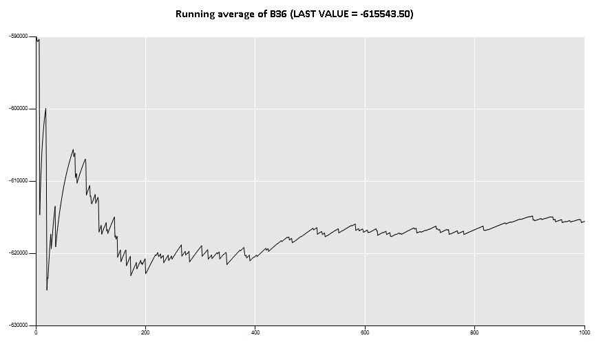
As we are expecting, the stochastic liability average is very close to the one calculated using the deterministic formula.
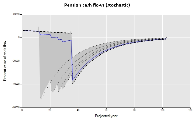
Now, the same kind of analysis can be made to get the projected cash flows. The charts below were built with the functions “sActuarialCashFlows” and “sActuarialRANDCashFlows” that receives the same inputs that the functions “sActuarialLiabilities” and “sActuarialRANDLiabilities”.
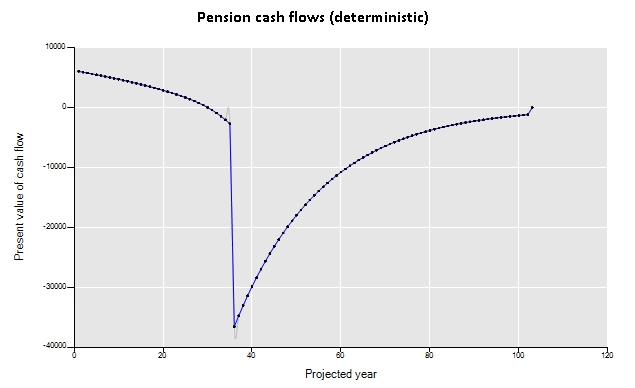
The stochastic chart was built using the time series simulation procedure, as explained here.