
Learning Center
How to perform a regression analysis?
Estimating relationships among variables is fundamental for econometricians. The Econometrics Toolbox was designed to deliver to you the analytical power of regression models right away at the tip of your fingers. Currently, SAFE TOOLBOXES® comes with the following regression models:
| # | Model Name | Model Description |
|---|---|---|
1 |
Linear |
The standard multivariate regression model. |
2 |
Logistic |
Logistic regression model. |
3 |
Binomial Logit |
A generalized regression model where the residuals follow a binomial distribution and the regressors connect to the dependent variable via the logit function (same as logistic). |
4 |
Binomial_Probit |
A generalized regression model where the residuals follow a binomial distribution and the regressors connect to the dependent variable via the probit function. |
5 |
Binomial_ComplementaryLogLog |
A generalized regression model where the residuals follow a binomial distribution and the regressors connect to the dependent variable via the complementary-log-log function. |
6 |
Poisson_Log |
A generalized regression model where the residuals follow a Poisson distribution and the regressors connect to the dependent variable via the log function. |
7 |
NegativeBinomial_Log |
A generalized regression model where the residuals follow a negative binomial distribution and the regressors connect to the dependent variable via the log function. |
8 |
Gamma_Reciprocal |
A generalized regression model where the residuals follow a gamma distribution and the regressors connect to the dependent variable via the function 1/x. |
9 |
InverseGaussian_ReciprocalSquared |
A generalized regression model where the residuals follow an inverse gamma distribution and the regressors connect to the dependent variable via the function 1/x^2. |
The last models belong to the generalized regression models class. Their names are constituted with two parts, the model family and the link function. The model family specifies the distribution of the errors in the dependent variable and the link function specifies the relationship between the dependent variable and the linear combination of predictor variables.
To fit a regression model in the Econometrics Toolbox you should write in the command window the name of the model followed by its equation. For the “linear” models, the standard regression model, the name of the model is not necessary and can be omitted. In the equation specification Y[] denotes the first time series selected, X1[] the second time series selected, X3[] the third, and so on.
A time series is presumed to be any contiguous range of numerical values in a column. Selecting a time series is done by selecting ONE cell in the series (can be any cell). To use a multivariate regression model you should press the CRTL key to allow you to select one cell for each series in your model.
In spite of we are using the term “time series” to denote a contiguous range of cells, it does not necessarily denote a series that is revealed as the time goes by. It can be any data series, like the final grades of students in class, the number of occurrences of a disease per country, etc.
There are also two special parameters to help you building your equation: the letter “C”, to represent the constant term in your model, or the word “TIME”, to include the time index of the series in your model, i.e., 1 for the first cell in your time series (counted from top to bottom direction), 2 for the second, etc.
Transformations of variables (log, exp, etc.) are also allowed to be used in your model. Transformations are inserted inside the brackets “[]” of variables. More than one transformation is permitted and they must be entered separated by a semicolon. A complete list of transformations and a detailed description of how to use them is explained here.
Categorical variables must be converted to numerical values before entering the model. A function “sTimeSeries_CategoricalToNumerical” can help you in this task. A categorical variable is a variable that represents states rather than a quantification. The states can be expressed by words (“good”, “normal”, “bad”/”cold”, “hot”/ “Before 1995”, “After 1995”, etc.) or numbers when they denote underlying states (1=good, 2=normal, 3= bad/1=”cold”, 2=“hot”/ 1=“Before 1995”, 2=“After 1995”, etc.) . The conversion function replaces the states by vectors of zeros and ones to indicate the presence of a given state in each time. One variable is discarded in the final matrix to avoid multicollinearity in your model. This discarded category can be seen as what happens if no one other states occur, i.e., when the row is zero for all other states. Finally, missing values (i.e., cells marked with an “*”) are well treated in the conversion as they reverberate in the respective lines of the final matrix.
All regression models are also available as Excel functions. For instance, you can use the function “sMultipleLinearRegression_Model” or “sLogisticRegression_Model” to fit the parameters under the “linear” or “logistic” model, respectively. Furthermore, in this examples, to recover the predicted values just call “sMultipleLinearRegression_Predicted” or “sLogisticRegression_Predicted” functions.
Now, to practice a little bit the concepts discussed above, we are going to build two regression models. First, a simpler one, with a standard multivariate regression model, and a more complex model, when we will use a logistic regression to build a credit analysis scoring system.
Example 1: Multivariate regression model
Consider that you want to build a multivariate linear regression model that follows the equation SeriesY = β0 + β1SeriesX1 + β2SeriesX2
A |
B |
C |
D |
E |
F |
|
1 |
Y Series |
X1 Series |
X2 Series |
|
|
|
2 |
104.7 |
3.3 |
2.8 |
|
|
|
3 |
657.4 |
37.8 |
10.2 |
|
|
|
4 |
211.8 |
12.8 |
7.1 |
|
|
|
5 |
1791.5 |
50.7 |
11.8 |
|
|
|
6 |
220.5 |
18.9 |
22.6 |
|
|
|
7 |
110.7 |
4.2 |
25.8 |
|
|
|
8 |
968.1 |
31.3 |
14.5 |
|
|
|
9 |
759.0 |
62.8 |
44.1 |
|
|
|
10 |
147.1 |
8.3 |
33.4 |
|
|
|
11 |
3575.2 |
76.1 |
28.9 |
|
|
|
12 |
981.5 |
33.2 |
28.5 |
|
|
|
13 |
2262.7 |
52.1 |
27.6 |
|
|
|
14 |
617.5 |
32.3 |
9.5 |
|
|
|
15 |
1408.1 |
43.8 |
8.3 |
|
|
|
16 |
362.2 |
19.6 |
2.5 |
|
|
|
17 |
195.4 |
11.7 |
34.4 |
|
|
|
18 |
3727.8 |
129.0 |
13.8 |
|
|
|
19 |
114.5 |
5.6 |
10.9 |
|
|
|
20 |
108.7 |
5.0 |
2.2 |
|
|
|
21 |
100.7 |
1.5 |
4.0 |
|
|
|
22 |
|
|
|
|
|
|
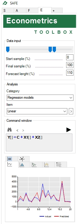
To perform multivariate regression, simply follow these steps:
- Select the Econometrics Toolbox tab;
- Select any cell containing the Y series (let’s say, cell A3) and press the CTRL key;
- Select any cell containing the X1 series (for instance, cell B5) and press the CTRL key;
- Select any cell containing the X2 series (for instance, cell C4);
- Adjust the start sample to 0% and the final sample to 100% (to use all 20 sample points);
- Set option Category = “Regression models” and item = “Linear” under the “Analysis” group and click on the button
 to confirm your choice. This will add the following equation in the command window: Y[] = C + X1[] + X2[]. Alternatively, you can just type the equation Y[] = C + X1[] + X2[] directly in the command window.
 - Click on the button
 , to run the regression.
Very simple, isn’t it? Now, let’s explore the results of our estimation in the tabs at the bottom at the Econometrics Toolbox tab.
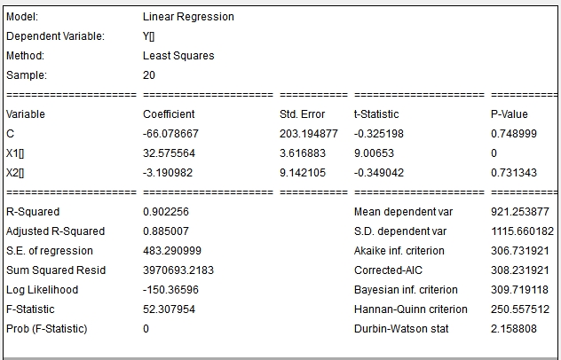
The model equation is found in the ![]() tab. When you double click it, a zoom of the table will pop up. In this table you can check the values of the fitted values for the parameters and some useful statistics, like the t-statistic of the independent variables, the R-Squared, the Akaike Information Criterion, etc.
tab. When you double click it, a zoom of the table will pop up. In this table you can check the values of the fitted values for the parameters and some useful statistics, like the t-statistic of the independent variables, the R-Squared, the Akaike Information Criterion, etc.
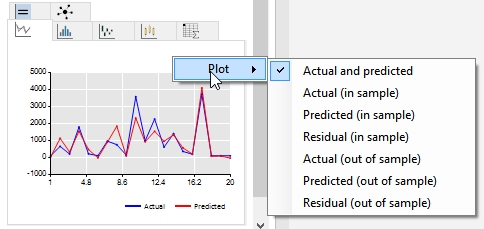
The line plot tab ![]() shows the dependent variable and the fitted dependent variable as default (see picture below). To change what this plot shows, right-click on it and select one of the available options: actual and predicted, actual (in-sample), predicted (in sample), residuals (in sample), actual (out of sample), predicted (out of sample) and residuals (out of sample). Only if you choose a final sample less than 100% (in step 5 above) you will be able to see the out of sample series represented in the chart. The out of sample period appears in the chart as a dotted line while the in sample period is represented by a continuous line.
shows the dependent variable and the fitted dependent variable as default (see picture below). To change what this plot shows, right-click on it and select one of the available options: actual and predicted, actual (in-sample), predicted (in sample), residuals (in sample), actual (out of sample), predicted (out of sample) and residuals (out of sample). Only if you choose a final sample less than 100% (in step 5 above) you will be able to see the out of sample series represented in the chart. The out of sample period appears in the chart as a dotted line while the in sample period is represented by a continuous line.
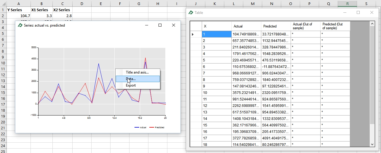
If you wish to access the values of the chart series, just right-click on it and select the option “Data…”.
To check the residuals density plot, select the density plot tab ![]() , right-click on it and select the “residuals (in sample)” option.
, right-click on it and select the “residuals (in sample)” option.

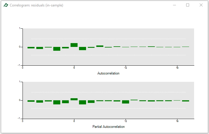
A similar procedure can be done to check if the residuals have any autocorrelation using the correlogram tab ![]() .
.
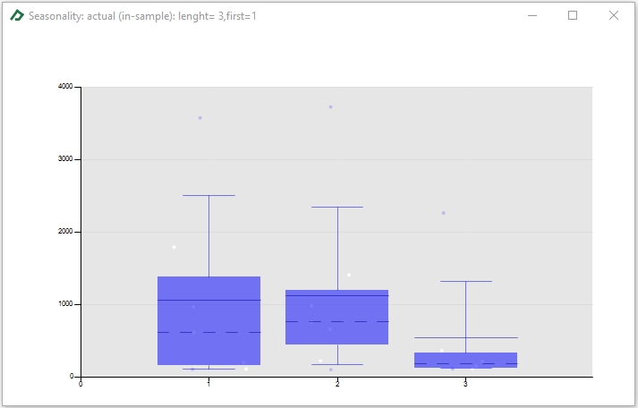
The box-plot tab ![]() allows you to check the presence of any seasonality in actual, predicted or residuals. Seasonality can be verified comparing if the centers of each box are aligned.
allows you to check the presence of any seasonality in actual, predicted or residuals. Seasonality can be verified comparing if the centers of each box are aligned.
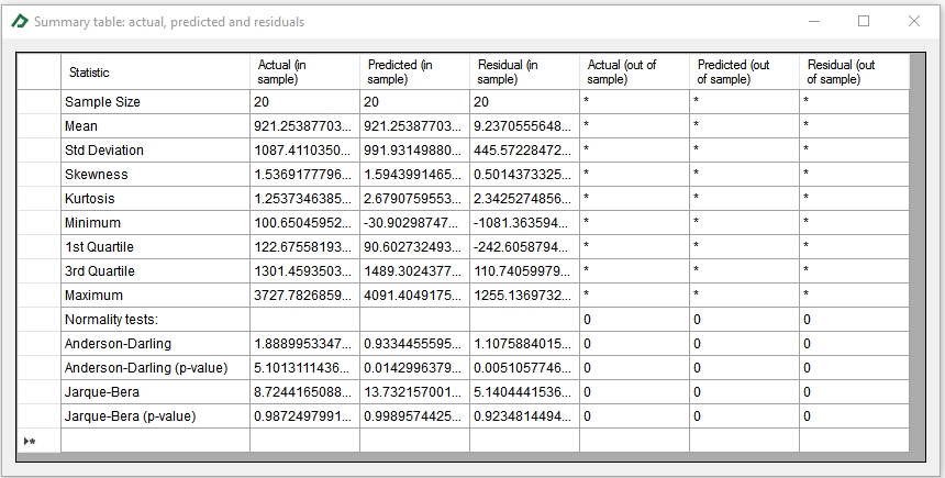
The summary tab ![]() provides the main descriptive statistics for the actual, predicted and residual series. In this table you can check, for instance, the Jarque-Bera or the Anderson-Darling tests for normality.
provides the main descriptive statistics for the actual, predicted and residual series. In this table you can check, for instance, the Jarque-Bera or the Anderson-Darling tests for normality.
Finally, the "Historical results” ![]() tab is populated each time that you run a model with main comparative statistics of your model. This tab is very useful when you want to explore different models for your data and select “the best one” using some statistics. For instance, you could select the best model as the one that has minimum Akaike Information Criterion or the higher Adjusted-R Squared.
tab is populated each time that you run a model with main comparative statistics of your model. This tab is very useful when you want to explore different models for your data and select “the best one” using some statistics. For instance, you could select the best model as the one that has minimum Akaike Information Criterion or the higher Adjusted-R Squared.

Example 2: Logistic regression model
The objective of this example is to show how to perform a logistic regression model to build a credit scoring model for a financial institution. Suppose, you have the following database containing some client’s financial ratios for each year and an indicator if it was on default (indicator= 0) that year or not (indicator= 1).
A |
B |
C |
D |
E |
F |
G |
H |
|
1 |
Credit database
|
|
|
|
|
|
|
|
2 |
|
|
|
|
|
|
|
|
3 |
Company ID |
Year |
Default |
WC/TA |
RE/TA |
EBIT/TA |
ME/TL |
S/TA |
4 |
1 |
1999 |
0 |
0.50 |
0.31 |
0.04 |
0.96 |
0.33 |
5 |
1 |
2000 |
0 |
0.55 |
0.32 |
0.05 |
1.06 |
0.33 |
6 |
1 |
2001 |
0 |
0.45 |
0.23 |
0.03 |
0.80 |
0.25 |
7 |
1 |
2002 |
0 |
0.31 |
0.19 |
0.03 |
0.39 |
0.25 |
8 |
1 |
2003 |
0 |
0.45 |
0.22 |
0.03 |
0.79 |
0.28 |
9 |
1 |
2004 |
0 |
0.46 |
0.22 |
0.03 |
1.29 |
0.32 |
10 |
2 |
1999 |
0 |
0.01 |
-0.03 |
0.01 |
0.11 |
0.25 |
11 |
2 |
2000 |
0 |
-0.11 |
-0.12 |
0.03 |
0.15 |
0.32 |
12 |
2 |
2001 |
0 |
0.06 |
-0.11 |
0.04 |
0.41 |
0.29 |
13 |
2 |
2002 |
0 |
0.05 |
-0.09 |
0.05 |
0.25 |
0.34 |
14 |
2 |
2003 |
0 |
0.12 |
-0.11 |
0.04 |
0.46 |
0.31 |
... |
... |
... |
... |
... |
... |
... |
… |
… |
3990 |
817 |
2001 |
1 |
0.23 |
-1.87 |
0.00 |
0.21 |
0.11 |
3991 |
818 |
1998 |
1 |
-0.21 |
-0.85 |
0.05 |
0.07 |
0.55 |
3992 |
819 |
1996 |
1 |
-0.12 |
-0.09 |
-0.01 |
0.14 |
0.34 |
3993 |
820 |
1996 |
1 |
0.24 |
-0.29 |
0.06 |
2.13 |
0.21 |
3994 |
821 |
2000 |
1 |
0.17 |
-0.26 |
0.03 |
0.03 |
0.19 |
3995 |
822 |
1998 |
1 |
-0.90 |
-0.52 |
0.04 |
0.03 |
0.59 |
3996 |
823 |
1997 |
1 |
0.30 |
0.03 |
0.03 |
0.04 |
0.57 |
3997 |
824 |
1996 |
1 |
0.41 |
-0.23 |
0.06 |
0.31 |
0.53 |
3998 |
825 |
1998 |
1 |
0.19 |
0.13 |
0.07 |
0.05 |
0.82 |
3999 |
826 |
1997 |
1 |
0.03 |
-1.85 |
0.03 |
0.03 |
0.68 |
4000 |
827 |
2000 |
1 |
0.17 |
-0.07 |
0.00 |
0.04 |
0.24 |
4001 |
828 |
1996 |
1 |
0.01 |
-0.26 |
0.04 |
0.30 |
0.15 |
4002 |
829 |
2001 |
1 |
-0.99 |
-0.43 |
0.00 |
0.04 |
0.33 |
4003 |
830 |
2002 |
1 |
0.07 |
-0.11 |
0.04 |
0.04 |
0.12 |
4004 |
|
|
|
|
|
|
|
|
To perform a logistic regression follows these steps:
- Select the Econometrics Toolbox tab;
- Select any cell containing the Y series (let’s say, cell C6) and hold the CTRL key;
- Select any cell containing the X1 series (for instance, cell D6);
- Select any cell containing the X2 series (for instance, cell E5);
- Select any cell containing the X3 series (for instance, cell F4);
- Select any cell containing the X4 series (for instance, cell G6);
- Select any cell containing the X5 series (for instance, cell H6);
- Adjust the start sample to 0% and the final sample to 100% (to use all 4000 sample points for estimation);
- Set option Category = “Regression models” and item = “Logistic” under the “Analysis” group and click on the button to confirm your choice. This will add the following text in the command window: Logistic: Y[] = X1[] + X2[]+ X3[] + X4[] + X5[]. Alternatively, you can just type the equation Logistic: Y[] = X1[] + X2[]+ X3[] + X4[] + X5[] directly in the command window.
- Click on the button , to run the regression.
Then, we will have the following equation of our model:
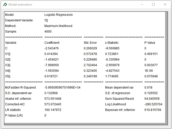
The logistic model will return the default probability for a given set of financial ratios of a company. So, for instance, if a company holds the indicators that appear in the last row of the database, the models predicts that there is a chance of 6.5% that it will default that year. Please note that after multiplying the equation coefficients by the financial ratios and founding Ŷ you must apply the link function that, in the case of the logistic regression, is the logit equation Z = 1/(1+exp(-Ŷ)).