
Learning Center
How to use Optimization Together with Simulation?
SAFE TOOLBOXES® comes with hundreds of functions to perform Monte Carlo Simulation that allow you to understand the range of all possible outcomes in your model. However, when your model also involves a decision process, you may also be interested in knowing which decision leads to the best range of outcomes. This class of problem is known by the name “optimization under uncertainty” and it is a major breakthrough in solving complex business problems.
An optimization together with simulation can be achieved with the following three steps:
- Step 1. Build your Simulation Model for an arbitrary fixed decision.
- Step 2. Compute the expectation of the variables of your interest using the “Data Table” approach.
- Step 3. Build your optimization model using Microsoft Solver.
A basic Asset and Liability Management will be presented below to illustrate how you can apply this technique to solve a chance-constrained optimization problem.
Simulation + Optimization: An Asset and Liability Management example
Suppose that a pension fund wants to minimize the chance that its assets will worth less than its liabilities over a 5-year horizon. The pension fund managers must decide the amount invested in bonds or stocks at the beginning of each year to face a fixed liability at the end of each year.
The managers projected that the pension fund assets and liabilities will evolve as presented below:
- Liabilities: Year 0 = $ 100, Year 1 = $ 106, Year 2 = $ 111, Year 3 = $ 115, Year 4 = $ 119, Year 5 = $ 123.
- Assets: Year 0: $100 (Initial amount to be invested).
- Bond’s returns follow a Vasicek model with parameters: Speed of mean reversion = 20%, Long-term interest rate = 4%, Volatility = 1%, Current interest rate = 3%.
- Stock’s returns follow a Geometric Brownian Motion model with parameters: Mean = 10%, Volatility = 20%.
So, the first step to build our simulation-optimization model is to create a Monte Carlo Simulation model for an arbitrary fixed decision. The spreadsheet below presents an implementation of such model with an equal amount invested in each asset class throughout the years:
|
A |
B |
C |
D |
E |
F |
G |
H |
1 |
A Chance-Constrained Asset and Liability Management example |
|
|
|||||
2 |
|
|
|
|
|
|
|
|
3 |
Time |
0 |
1 |
2 |
3 |
4 |
5 |
|
4 |
Assets |
100.0 |
102.0 |
109.0 |
118.6 |
141.1 |
156.8 |
<=G5+G6 |
5 |
Bonds |
|
51.7 |
52.2 |
55.5 |
60.3 |
73.0 |
<=F4*G16*(1+G12) |
6 |
Stocks |
|
50.3 |
56.9 |
63.1 |
80.8 |
83.8 |
<=F4*G17*(1+G13) |
7 |
Liabilities |
100.0 |
106.0 |
111.0 |
115.0 |
119.0 |
123.0 |
|
8 |
Coverage ratio (Assets/Liabilities) |
1.00 |
0.96 |
0.98 |
1.03 |
1.19 |
1.27 |
<=G4/G7 |
9 |
Coverage ratio <1? |
0 |
1 |
1 |
0 |
0 |
0 |
<=IF(G8<1,1,0) |
10 |
Coverage Ratio Indicator |
1 |
<=IF(SUM(B9:G9)>0,1,0)+ B22*0 |
|
|
|
|
|
11 |
|
|
|
|
|
|
|
|
12 |
Bond returns (Vasicek Model) |
3.0% |
3.4% |
2.3% |
1.9% |
1.6% |
3.5% |
<=sInterestRatesVasicek_RAND(20%,4%,1%,F12,1) |
13 |
Stock returns (MGB Model) |
|
0.5% |
11.5% |
15.7% |
36.2% |
18.8% |
<=sRAND_Lognormal(10%,15%)-1 |
14 |
|
|
|
|
|
|
|
|
15 |
Decision variables (Proportion of bonds) |
|
|
|
|
|
|
|
16 |
Bonds |
|
50% |
50% |
50% |
50% |
50% |
|
17 |
Stocks |
|
50% |
50% |
50% |
50% |
50% |
<=1-G16 |
18 |
|
|
|
|
|
|
|
|
As you may have noticed, the formula in cell B10 represents an indicator about the achievement of our goal in a given scenario/decision. The indicator will be valued with “0” if the value of the assets is greater than the liabilities during all five years and will be “1” if the value of the assets is less than the liabilities for at least one year.
Now that our Simulation Model is completed, we can go to the second step of our simulation-optimization model, where we compute the expectation of our interest variable using the “Data Table” approach.
In our ALM problem, we want to compute the expected value of our indicator to get the chance of not achieving our goal, given that we have made a particular set of decisions. So, to get an approximation of this probability based on a 1,000 sample using the Data Table approach , just follow the steps below:
- Create a table as follows: enter a sequence from 1 to 1000 in cells A25:A1024 and put the formula "=B10" in cell B24.
- Select the range A25:B1024, go to Data > What-if analysis > Data table… and type B22 in the “Column input cell” field. The simulation of the indicator will be displayed in cells B25:B1024.
- Compute the expected value using the Excel’s average formula in cell B21.
|
A |
B |
C |
D |
E |
F |
G |
H |
14 |
|
|
|
|
||||
15 |
Decision variables (Proportion of bonds) |
|
|
|
|
|
|
|
16 |
Bonds |
|
50% |
50% |
50% |
50% |
50% |
|
17 |
Stocks |
|
50% |
50% |
50% |
50% |
50% |
<=1-G16 |
18 |
|
|
|
|
|
|
|
|
19 |
Data Table Monte Carlo Simulation |
|
|
|
|
|
||
20 |
|
|
|
|
|
|
|
|
21 |
Expected value of Coverage Ratio Indicator |
60,3% |
<=AVERAGE(B25:B324) |
|
|
|
|
|
22 |
Number to force calculation |
0.378114424 |
<=RAND() |
|
|
|
|
|
23 |
|
|
|
|
|
|
|
|
24 |
|
1 |
<=B10 |
|
|
|
|
|
25 |
1 |
0 |
|
|
|
|
|
|
26 |
2 |
1 |
|
|
|
|
|
|
27 |
3 |
1 |
|
|
|
|
|
|
… |
… |
… |
… |
… |
… |
… |
… |
… |
1020 |
996 |
1 |
|
|
|
|
|
|
1021 |
997 |
0 |
|
|
|
|
|
|
1022 |
998 |
1 |
|
|
|
|
|
|
1023 |
999 |
0 |
|
|
|
|
|
|
1024 |
1000 |
1 |
|
|
|
|
|
|
1025 |
|
|
|
|
|
|
|
|
Here we can see that holding the 50-50 mix of bonds and stocks will lead to a 60.3% chance of mismatching. How to minimize this probability by changing the assets proportions is the last step in our simulation and optimization approach.
To set up the optimization model go to Solver (it should be enabled in Excel’s options to appear in the Ribbon) and fill in the form as displayed in the picture below.
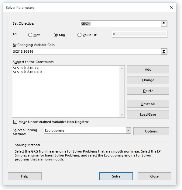
One important parameter is the selection of the solver to be used. As a rule of thumb, you can try the “Generalized Non-linear” first as it's the fastest one, but it only works with smooth functions (which is generally not the case in simulation optimization problems!). Normally the “Evolutionary Solver” will be your unique possible choice. Nevertheless, it has a disadvantage of being a very slow procedure that produces only satisfactory results (as you can never know if a global optimal was achieved).
By solving our optimization problem, we can see that the solution found reduced the chance of mismatching from 60.3% to 46.0%. This result is achieved with the following allocations:
|
A |
B |
C |
D |
E |
F |
G |
H |
14 |
|
|
|
|
||||
15 |
Decision variables (Proportion of bonds) |
|
|
|
|
|
|
|
16 |
Bonds |
|
4% |
39% |
89% |
62% |
66% |
|
17 |
Stocks |
|
96% |
61% |
11% |
38% |
34% |
<=1-G16 |
18 |
|
|
|
|
|
|
|
|
19 |
Data Table Monte Carlo Simulation |
|
|
|
|
|
||
20 |
|
|
|
|
|
|
|
|
21 |
Expected value of Coverage Ratio Indicator |
46.0% |
<=AVERAGE(B25:B324) |
|
|
|
|
|
Please note that the results of our simulation-optimization model can differ a little each time that we run our model as we are using a simulation procedure and a non-deterministic optimization method to solve the problem.