Learning Center

How to use Support Vector Machines for classification or regression?

Support Vector Machines (SVM) are algorithms that have shown very promising results in classification and regression problems. This machine learning technique has a wide range of applications in finance, such as bankruptcy prediction and financial time series forecasting.

SAFE TOOLBOXES® comes with functions to cope with binary classification problems, where values “-1” and “1” are used to label the classes in the dependent variable, and regression problems, where the dependent variable has a real value domain.

To illustrate the usage of this tool, examples of classification and regression models are presented below:

Example 1

Using Support Vector Machines for classification

Example 2

Using Support Vector Machines for regression

Example 1: Using Support Vector Machines for classification

Suppose that you want to forecast if the next year return of a given stock will be higher than 5% (labeled with “+1” class, and “-1” otherwise) based on some company’s historical financial ratios, as presented in the spreadsheet below:

The first step is to estimate your SVM model using the function called “sMachineLearning_SupportVectorMachine_Model”. This function takes the following five parameters:

• DataMatrix: The range of your training set. The dependent variable must be placed in the first column followed by the set of explanatory variables.
• VariableNames: A vector containing the names of dependent and explanatory variables.
• ErrorPenaltyValueOrVector: A value that penalizes wrong classifications. You can also enter a vector to associate a different penalty for each sample misclassification.
• KernelName: A string with the name of the chosen kernel (consult the table below to see the list of available kernels). In short, a Kernel is a transformation of the explanatory variables set to improve the prediction power.
• KernelVectorOfParameters: A vector containing the parameters of the Kernel (consult the table below to see the order of parameters).

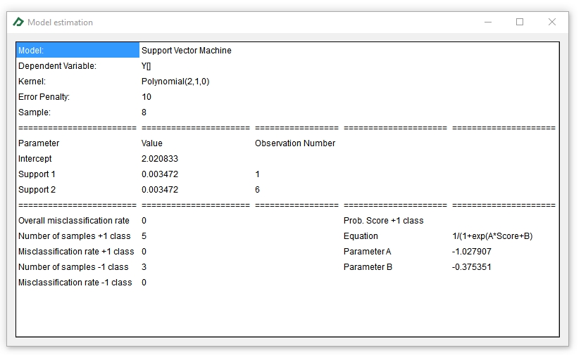
Let’s suppose that we want to use the Polynomial[2,1,0] Kernel. To do that, just enter the formula “=sMachineLearning_SupportVectorMachine_Model(C4:E11,C3:E3,10,B15,B16:D16) “ in cell A18 and press the MVF button . You will get the following result:

Finally, to perform the SVM forecast, you can type the following formulas in cells F4, G4 and H4:

• SVM “+1” and “-1” classification prediction (cell F4 + MVF button ): “=sMachineLearning_SupportVectorMachine_Predicted(D4:E12,"Classification",C4:C11,D4:E11,B26:B27,C26:C27,B25,B15,B16:D16)”
• SVM raw score prediction (cell G4 + MVF button ): “=sMachineLearning_SupportVectorMachine_Predicted(D4:E12,"Score",C4:C11,D4:E11,B26:B27,C26:C27,B25,B15,B16:D16)”. Please note that a positive score means a “+1” classification, while a negative score leads to a “-1” classification.
• SVM probability of being a “+1” class (cell H4): “=1/(1+EXP($E$31*G4+$E$32))”

Hint: The usage of the scores can be helpful when you have more than two categorical variables. In this case, you can compute multiples SVM models (for instance, Model 1: use “+1” for category A and “-1” otherwise, Model 2: use “+1” for category B and “-1” otherwise, etc.) and, then, attribute the category to a given sample based on the highest score computed among the models.

By entering the formulas above, you will get the following result:

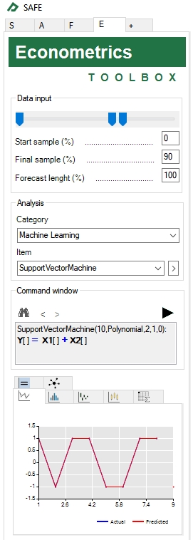
Finally, you can use the Econometrics Toolbox to estimate your model directly from the spreadsheet. To do this, just perform the following steps:

1. Select the Econometrics Toolbox tab.
2. Select any cell containing the c_t+1 series (let’s say, cell C4) and press the CTRL key.
3. Select any cell containing the ROE_t series (for instance, cell D4) and press the CTRL key.
4. Select any cell containing the d_t series (for instance, cell E4).
5. Adjust the training sample size to estimate the model in the “Data input” pane. In our example, you should enter 90% in the final sample to get the “C4:E11” range (i.e., to use all 8 samples for the training set ) and 100% in the forecast length to make a prediction for the training set and for the out-of-sample point in range “D12:E12”.

Hint: Please note that you can use the button to check the range used for estimation and prediction based on the information you provided in the “data input” pane.

6. Set option Category = “Machine Learning” and item = “Support Vector Machine” under the “Analysis” group and click on the button to confirm your choice. This will add the following equation to the command window: “SupportVectorMachine(ErrorPenaltyValue,KernelName,KernelParam1,KernelParam2,KernelParam3): Y[] = C + X1[] + X2[]”.
7. To input the parameters of the model modify the formula “SupportVectorMachine(ErrorPenaltyValue,KernelName,KernelParam1,KernelParam2,KernelParam3): Y[]= C + X1[] + X2[]” to “SupportVectorMachine(10,Polynomial,2,1,0): Y[] = X1[] + X2[] ”.
8. Click on the button to run the model.

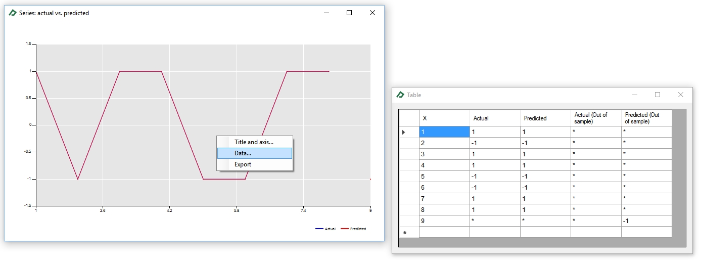
The model estimation table will appear on the Model Estimation tab .You could double-click the table to get an enlarged view of it.

The observed and predicted categories can be seen in the Line Chart tab . To check the values, double-click the chart and then select the option “Data...” after right-clicking the zoomed the chart.

Example 2: Using Support Vector Machines for regression

Performing an SVM regression using SAFE TOOLBOXES® is a quite similar procedure to running an SVM classification (in fact, all SAFE TOOLBOXES® estimation and prediction models follow similar steps). You can either estimate the SVM regression using spreadsheet functions or by the “Command Window” tool.

To illustrate the usage of this tool, suppose that we want to forecast the stock returns using its own lagged values, as presented in the spreadsheet below:

To compute the Support Vector Machine Regression model, type in cell A18 the formula “=sMachineLearning_SupportVectorRegression_Model(B4:D12,B3:D3,10,2%,B15,B16:D16)” and then press the MVF button to get all table values. The formula parameters are described below:

• DataMatrix: Series with the dependent variable in the first column followed by the regressors series.
• VariablesNames: Regressors names.
• ErrorPenaltyValueOrVector: The penalty value or vector associated with each error.
• NonPenalizedErrorSize: The amount of error that won't be penalized.
• KernelName: The name of the chosen Kernel. See the Kernels Table.
• VectorOfParameters: The vector of parameters associated with the chosen Kernel. See the Kernels Table.      

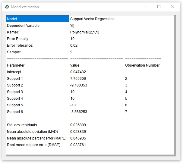
And the resulting model table will look like this one:

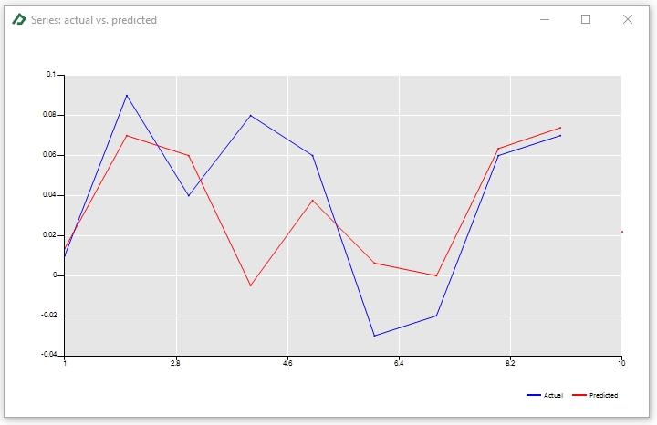
Finally, to get the prediction, just type the formula “=sMachineLearning_SupportVectorRegression_Predicted(C4:D13,C4:D12,B27:B32,C27:C32,B26,B15,B16:D16)” in cell “E4” and press the MVF button . You will see the following result:

To do the same analysis by the “Command window” tab, please follow these steps:

1. Select the Econometrics Toolbox tab.
2. Select any cell containing the R_t series (let's say, cell B4) and press the CTRL key.
3. Select any cell containing the R_t-1 series (for instance, cell C6) and press the CTRL key.
4. Select any cell containing the R_t-2 series (for instance, cell D5).
5. Adjust the start sample to 0%, the final sample to  90% and the forecast length to 100% (to use the first 9 sample points for the training set and to predict from year 1 to 10).
6. Set option Category = “Machine Learning” and item = “Support Vector Regression” under the “Analysis” group and click on the button to confirm your choice. This will add the following equation in the command window: "SupportVectorRegression(ErrorPenaltyValue,NonPenalizedErrorSize,KernelName,KernelParam1,KernelParam2,KernelParam3): Y[] = X1[] + X2[]".
7. Replace the above equation to "SupportVectorRegression(10,0.02,Polynomial,2,1,1): Y[] = X1[] + X2[]" to input the parameters of the model.
8. Click on the button to run the regression.

At the bottom of the Econometrics Toolbox tab you will get many interesting results, as the Actual x Predicted chart and the Model Table displayed below: